Building a calibrated gene tree with BEAST 2.7 |

Since our blog is called The BEAST, it is only fair that we debut our posts by discussing Bayesian Evolutionary Analysis Sampling Trees, or simply BEAST (Bouckaert et al. 2019), one of the most widespread molecular phylogenetic software packages. Although there are many great tutorials on the BEAST2 website and even an entire site dedicated to a yearly course taught by some of the developers (see Taming the BEAST), I believe that a step-by-step guide aimed at new users is always welcome.

In Bayesian phylogenetic analyses, hypotheses (i.e., the tree and its parameters) are generated based on a data matrix, an assumed model of nucleotide evolution, and various priors. We will revisit all of this shortly, but for now, we will need a molecular matrix. For this, we will use the 16S mtDNA matrix from the description of Pristimantis rupicola (Anura: Brachycephaloidea), from Taucce et al. (2020). I will assume you are familiar with retrieving sequences from GenBank and aligning them, but we will cover these topics in future posts.

BEAST2 interprets XML files, and to build one, we will use the BEAUti app, which is part of BEAST software package. First, we will load our molecular matrix by going to File > Import Alignment. BEAUti will prompt us to specify the type of data we have, and we will select “nucleotide” (Fig. 1).

**Figure 1:** BEAUti screen after you have loaded the molecular matrix.

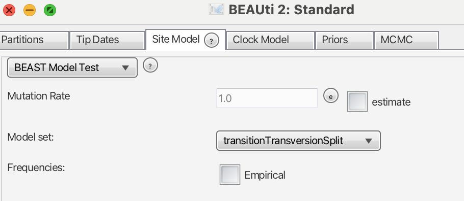
We will leave the “Tip Dates” panel as it is and move on to the “Site Model” panel (Fig. 2). At this stage, we need to select a nucleotide substitution model for our data. While there are several software packages available for this task, BEAST conveniently includes an inbuilt package that will infer the best-fitting nucleotide substitution model simultaneously with the phylogenetic tree inference: bModelTest (Bouckaert & Drummond, 2017). If the BEAST Model Test option is not available, you may need to install it by navigating to File > Manage Packages. With that in place, we are now ready to proceed to the next panel, “Clock Model.”

**Figure 2:** Site Model tab showing the use of the bModelTest package.

When we open the panel, the strict clock model is already selected. This model assumes that the clock rate evolves equally across the entire tree. However, since our matrix involves interspecific relationships, this assumption is likely not suitable. We could test how “clock-like” our data are, but that will be the subject of a future post. For now, it is advisable to choose the “optimised relaxed clock model”.

There are two main ways to date a phylogenetic tree: either by assigning ages to the nodes, usually based on geological events or fossil records, or by specifying a clock rate—i.e., informing BEAST of the nucleotide substitution rate in our matrix. While it is common practice to use a single predetermined clock rate from the literature, we will take a different, more elegant approach. Since it is unlikely that the same clock rate applies to different datasets, estimating the rate is more appropriate. However, to ensure plausible results and aid the analysis in converging, it is recommended to introduce a narrow prior. But how do we do that?

According to Drummond & Bouckaert (2015), if “a number of independent rate estimates from other papers on relevant taxa and gene regions” are available, one can fit a log-normal distribution to these values and use them as a prior. Since several estimates for the 16S gene in frogs are available in the literature (see Lemmon et al., 2007, Fouquet et al., 2012, Gehara et al., 2017, and Dufresnes et al., 2022), we will follow this approach. All we need is R (R Core Team, 2024) and a small piece of code:

library(fitdistrplus)
library(stats)

rate <- c(0.006, 0.00555, 0.00277, 0.005)  # Define a vector of rates
ratedist <- fitdist(rate, "lnorm")  # Fit a log-normal distribution to the rate data

mean <- mean(rate)  # Calculate the mean of the rates, it will be useful as a starting point
log.mean <- unname(ratedist$estimate["meanlog"])  # Get the estimated mean value from the fitted lognormal distribution
log.sd <- unname(ratedist$estimate["sdlog"])  # Get the estimated sd value from the fitted lognormal distribution

In our case, the mean of the log-normal distribution is -5.374295 and the sd is 0.304072. We will use hese values in the “Priors” panel shortly. For now, let’s use the mean of our four rate values, 0.00483, as a starting point to help the Markov chains converge (Fig. 3). Do not forget to check the “estimate” box. To do this, navigate to Mode and uncheck the Automatic set clock rate option.

**Figure 3:** Clock Model panel showing the chosen model, Optimised Relaxed Clock, and the starting value of the `clock.rate` prior.

Moving on to the “Priors” panel, we will see several parameters. We will leave most of them under default, but we will change the tree and the molecular clock priors. The current tree prior, “Yule”, has only one parameter to be estimated, the birth rate, assuming no extinction events. A more appropriate prior would be the Birth Death Model (Fig. 4), which does account for extinction.

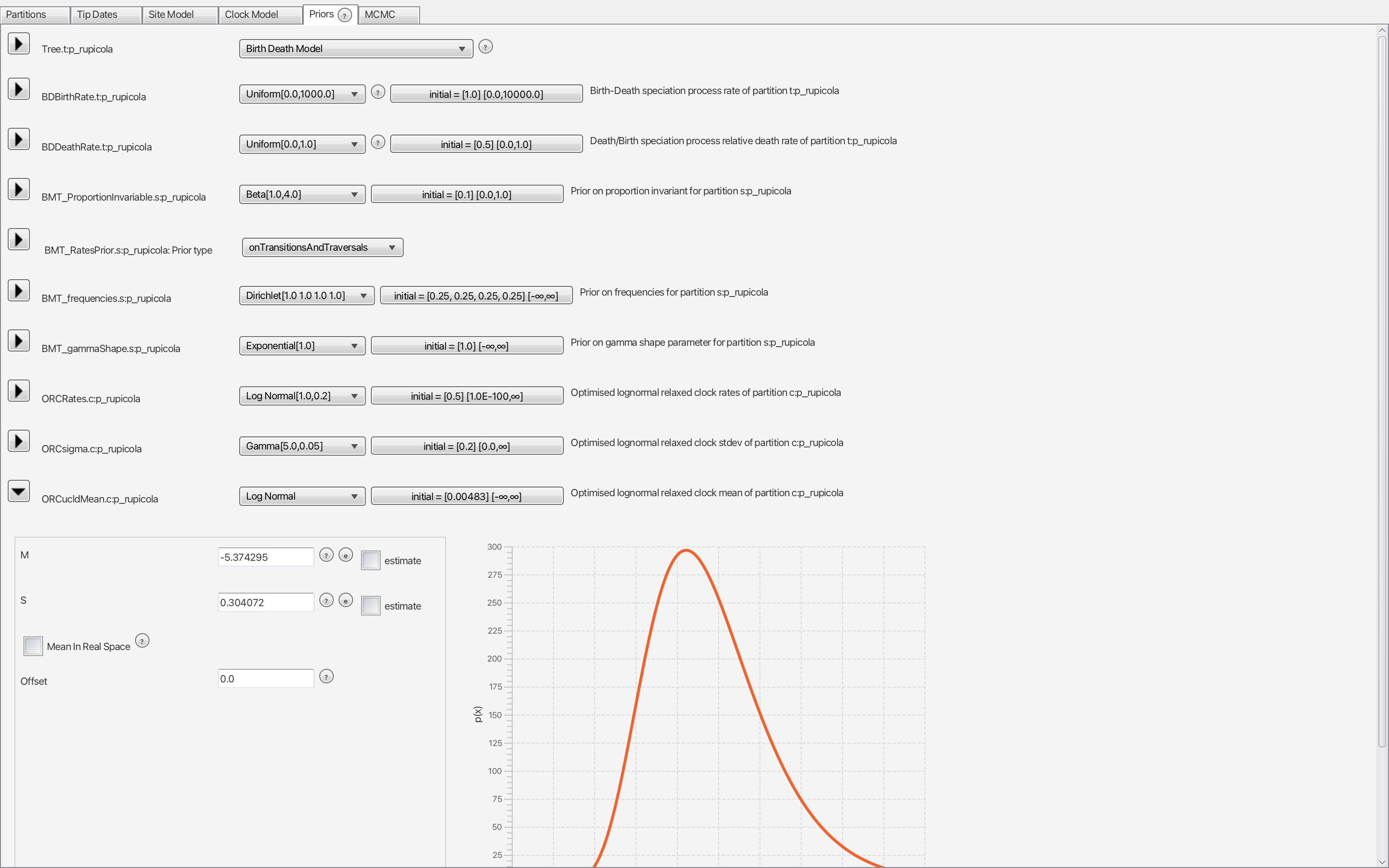
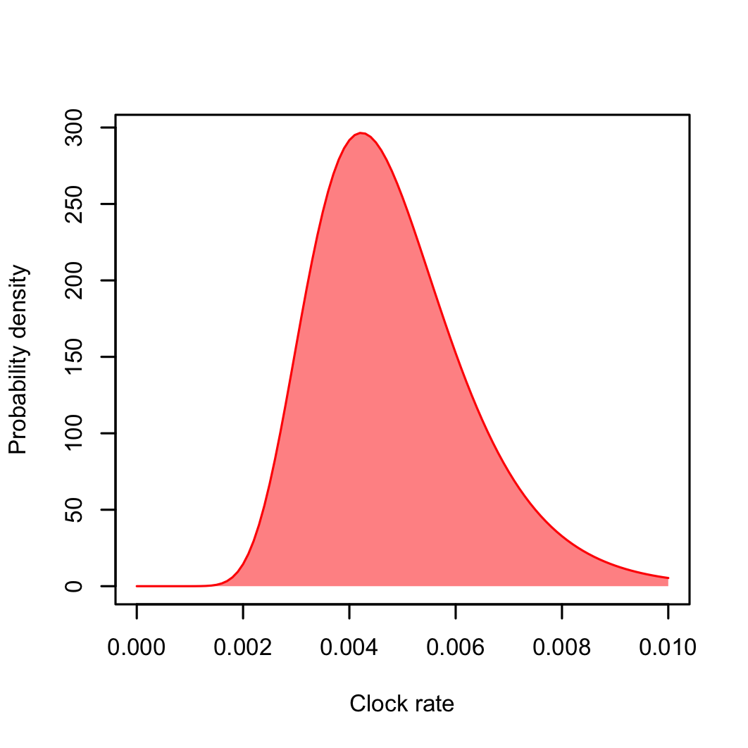
**Figure 4:** Priors panel, showing the changes in tree and ORCucldMean models.

Finally, we are going now to use the mean and standard deviation we calculated from our log-normal model. Open the ORCucldMean.c prior and add the meanlog value (in our case, -5.374295) to the M parameter and sdlog (0.304072) to S (Fig. 4). To make sure, you can plot your log-normal model and compare it to the one in BEAUti (Fig. 5):

x <- seq(0, 0.01, length = 100)  # Create a sequence of values from 0 to 0.01 with 100 points
y <- dlnorm(x, meanlog = log.mean, sdlog = log.sd)  # Calculate the density of the log-normal distribution for the x values

# Set up the graphics device to save the plot as a PNG file
png("your_path.png", width = 90, height = 90, units = "mm",
    res = 300, pointsize = 8)

# Plot the density curve of the log-normal distribution
curve(dlnorm(x, meanlog = log.mean, sdlog = log.sd), ylab = "Probability density",
      from = 0.001, to = 0.01, col = "red", xlab = "Clock rate", lwd = 1)

# Add a filled polygon under the density curve
polygon(c(x, rev(x)), c(y, rep(0, length(y))), col = rgb(1, 0, 0, 0.5), border = NA)

dev.off()  # Close the graphics device

**Figure 5:** Plot of the fitted log-normal model

We will leave the MCMC panel unchanged. If your dataset is larger, you may want to consider increasing the number of generations, but for our matrix, 10 million generations with sampling every 1,000 generations should be sufficient.

Results

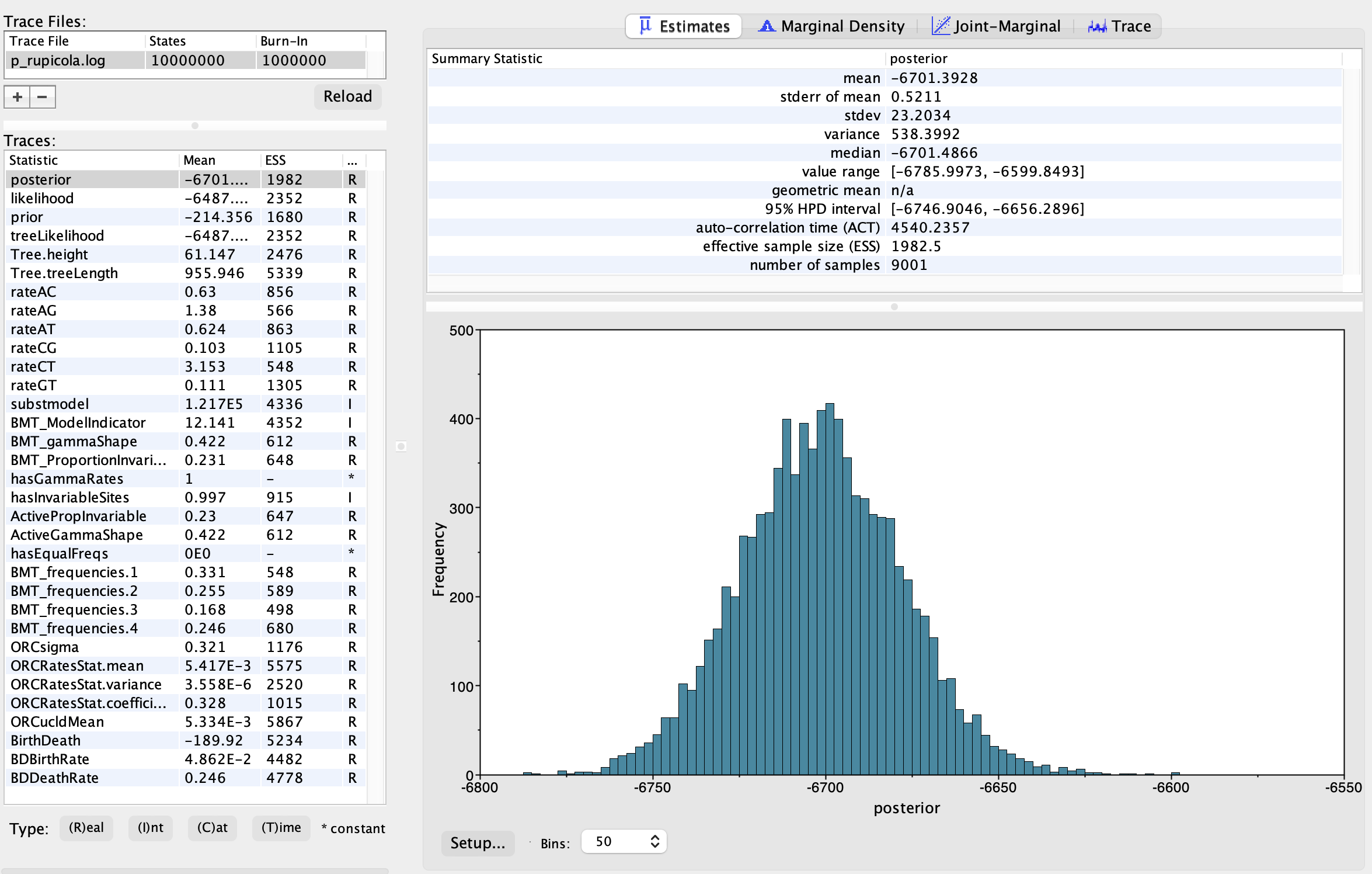
We will use Tracer (Rambaut et al., 2018) to assess the convergence of the MCMC output. Ideally, all ESS values should exceed 200. When conducting the final analysis, you should run at least one additional replicate, starting from a different seed, to ensure that the MCMC has fully converged.

To check our analysis, click the “+” button in the top left corner and load the .log file generated by BEAST. As shown in Fig. 6, a chain length of 10,000,000 generations was sufficient for the MCMC output to converge.

**Figure 6:** Tracer output after loading the log file.

The .trees files generated by BEAST contain multiple trees, representing the posterior distribution from the Bayesian analysis. We will now summarize these into a Maximum Credibility Tree using another BEAST tool, TreeAnnotator. The only change I will make is regarding node heights, which I will set to “mean heights”—but feel free to use the option that best suits your analysis (Fig. 7).

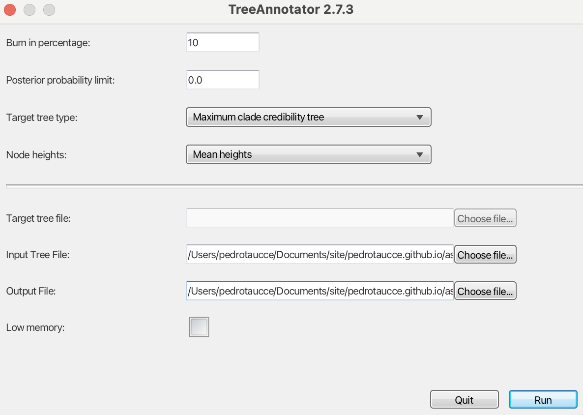
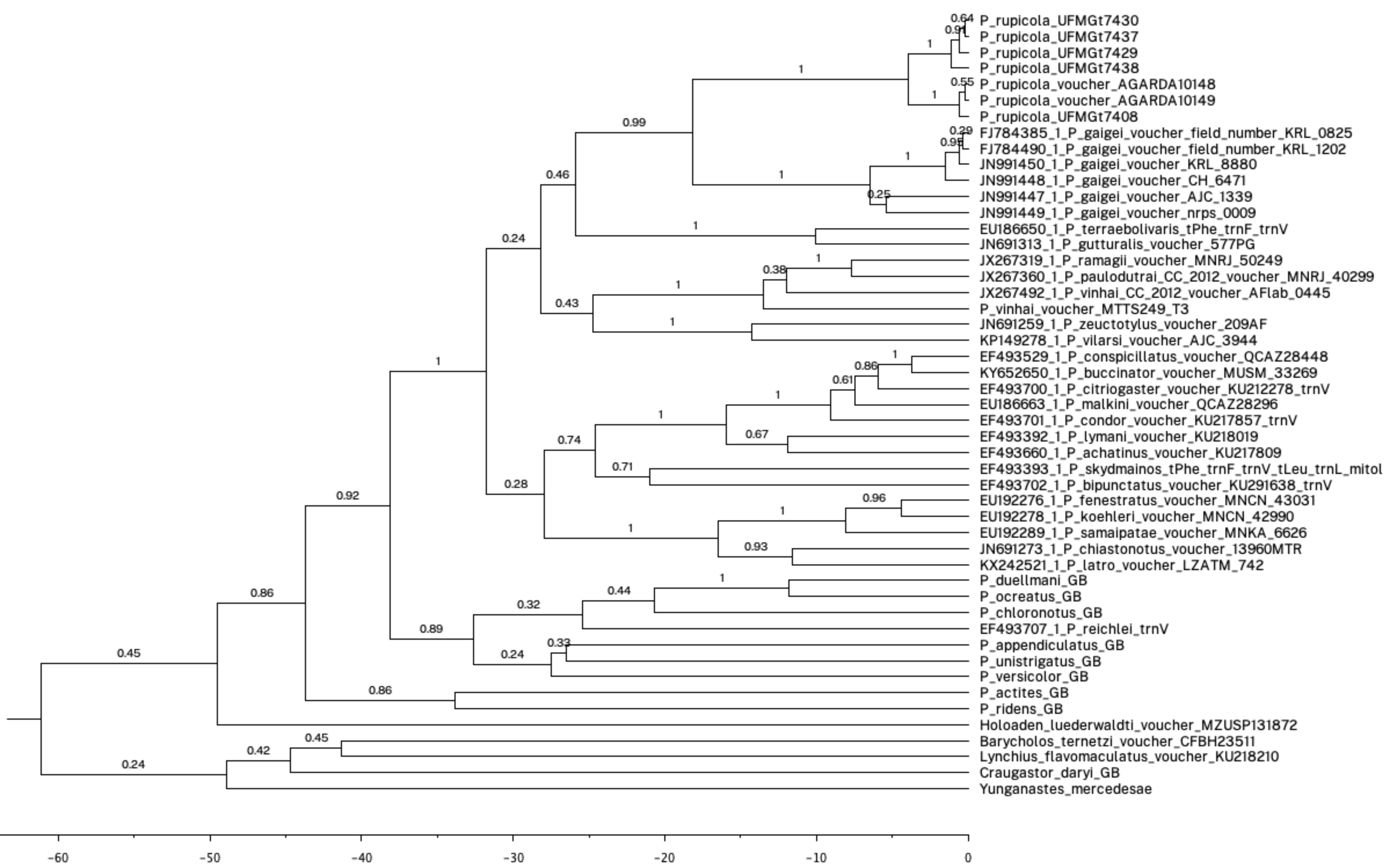
**Figure 7:** TreeAnnotator window with node heights set to "mean heights".

After adjusting the input to your .trees file and naming the output as you prefer, you can view the results using your favorite tree viewer. I hope your output looks as cool as mine (Fig. 8)!

**Figure 8:** Chronogram of 16S showing the relationships within *Pristimantis* species.

References

Bouckaert, R., & Drummond, A. J. (2017). bModelTest: Bayesian phylogenetic site model averaging and model comparison. BMC Evolutionary Biology, 17(1), 42.

Bouckaert, R., Vaughan, T. G., Barido-Sottani, J., Duchêne, S., Fourment, M., Gavryushkina, A., et al. (2019). BEAST 2.5: An advanced software platform for Bayesian evolutionary analysis. PLoS Computational Biology, 15(4), e1006650.

Dufresnes, C., Mahony, S., Prasad, V. K., Kamei, R. G., Masroor, R., Khan, M. A., … Litvinchuk, S. N. (2022). Shedding light on taxonomic chaos: Diversity and distribution of South Asian skipper frogs (Anura, Dicroglossidae, Euphlyctis). Systematics and Biodiversity, 20(1), 1–25.

Fouquet, A., Noonan, B. P., Rodrigues, M. T., Pech, N., Gilles, A., & Gemmell, N. J. (2012). Multiple Quaternary refugia in the eastern Guiana Shield revealed by comparative phylogeography of 12 frog species. Systematic Biology, 61(3), 461.

Gehara, M., Barth, A., de Oliveira, E. F., Costa, M. A., Haddad, C. F. B., & Vences, M. (2017). Model-based analyses reveal insular population diversification and cryptic frog species in the Ischnocnema parva complex in the Atlantic forest of Brazil. Molecular Phylogenetics and Evolution, 112, 68–78.

Lemmon, E. M., Lemmon, A. R., & Cannatella, D. C. (2007). Geological and climatic forces driving speciation in the continentally distributed trilling chorus frogs (Pseudacris). Evolution, 61, 2086–2103.

R Core Team (2024). R: A language and environment for statistical computing. R Foundation for Statistical Computing, Vienna, Austria.

Taucce, P. P. G., Nascimento, J. S., Trevisan, C. C., Leite, F. S. F., Santana, D. J., Haddad, C. F. B., & Napoli, M. F. (2020). A new rupicolous species of the Pristimantis conspicillatus group (Anura: Brachycephaloidea: Craugastoridae) from Central Bahia, Brazil. Journal of Herpetology, 54(2), 245–257.